


 | Next: Bibliography |
Aims:
Disadvantages:
The previous considerations of the logistic concept where more of a
technical nature: which module is doing what and exchanging which
information with other modules.
Assumptions:
Advantages:
Possibility of sub-optimum operation compared with a completely
deterministic approach.
In the sequel we discuss methods on
The random buffered network model
A buffer can be any track element , such as
lines, stops, carrier exchanger, or cabin and carrier stores.
Property:
![]() ,
where
,
where
![]() is randomly distributed with
the probability density function
is randomly distributed with
the probability density function
![]() .
.

Each estimation is based on a model that represents the reality
``good enough'' for the purpose of the respective estimation. Other
models may be more realistic, but more difficult to
analyse and to compute.
The probability density function
![]() could also depend
on other parameters
could also depend
on other parameters
![]() that are known or can be estimated at time
that are known or can be estimated at time
![]() such
that the characteristics of the buffer are determined by
such
that the characteristics of the buffer are determined by
Examples of
![]() for different buffer types:
for different buffer types:
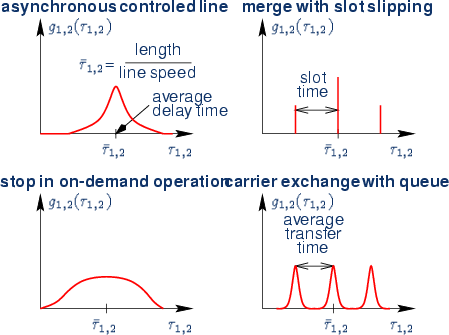
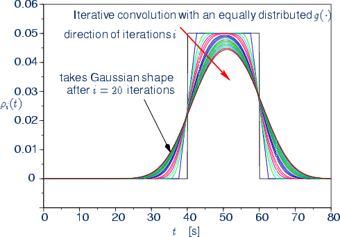
Then the I/O behavior is characterized by the convolution
The convolution
Assumption: the entrance time t1 of cabin or carrier is
random and represented by the probability density function
![]() .
.


![]() is only valid if
is only valid if
![]() and
and
![]() are
statistically independent, which is a reasonable assumption.
are
statistically independent, which is a reasonable assumption.
The Input-Output behavior of the buffer chain is characterized by
Average arrival time
Variance

![]()
![]() at connecting point c:
at connecting point c:
![]()
![]() of arrival time tc at connecting
point c:
of arrival time tc at connecting
point c:
![]()
where
![]() is the variance of
is the variance of
![]() .
.
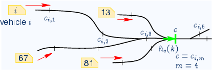
Example of network model for cabins
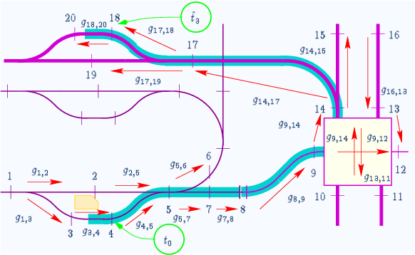
Estimated arrival time:
Variance of estimated arrival time:
The predictions are time discretized in time slots of duration T.
The duration T depends on the dynamics on a specific track
element.
The probability
pi,m(k) that vehicle i enters
connecting point ci,m during the time slot k is
determined by

where
![]() is the probability density function of
vehicle i at connecting point ci,m .
is the probability density function of
vehicle i at connecting point ci,m .

Time slots is a concept that is know in air-traffic control: the air traffic controller (which are still humans) assign a time-slot to each airplane, that wants to start or land, whereby one airplane is assigned to one times-lot. For the PSNC we want to automate this process, and a first step is to estimate the probability that a vehicle occurs in a certain time-slot at a certain place. The difference between PSNC and the air traffic control is that we can enlarge the time interval of a time slot and allow multiple vehicles to occupy it. The exact sequence of the vehicles and the distance between the vehicle is then a task of the local control subsystem and depends on the carrier-track technology. Also in case of an over-assignment by the logistics, the local control subsystem needs to deviate vehicles or, if necessary, slow them down in order to prevent an emergency break. However, the probability of that event can be reduced arbitrarily (as shown later on). In case of such a buffer-overflow, all concerned vehicles will make the transient from a the nominal operation to a steady state. The user in the vehicles will not notice this transition because all comfort criteria will be respected. However, he may notice that his vehicle will not take the shortest way. The concerned vehicles will flip back to nominal operation as soon as their trip has been rerouted and reallocated.
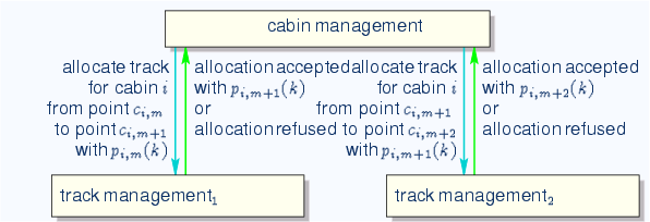
PSNC for track allocation
Simple analogy:
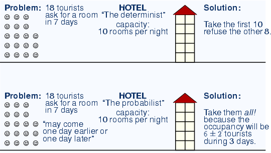
The analogy with the hotel reservation illustrates the problem of probabilistic slot allocation. With a hotel, one time slot corresponds to one night and the hotel capacity (here 10 persons) corresponds to the maximum number of vehicles allowed per time slot.
|
Controlled quantities: using the random buffer network model, it is necessary to control two critical quantities for each buffer:
|
|
Aim:
|
 |
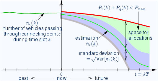
In the hotel-example before, we assumed that the hotel were completely empty for that concerned day. However, there may also be some guests that have been there before. This cumulative quantity is defined by q1,2(k). Another difference is that a hotel is usually not limited by the influx of people, as long as the reception can handle all arriving or leaving guests before closing. A transport network, where all guideways have a limited carrying capacity this flux (vehicles entering n1(k) or leaving n2(k) per time-slot) needs also to be taken into consideration. In the following we determine the estimations of future q1,2(k), and n1(k) and thereafter propose a possible criteria on how to decide whether or not to grand an allocation.
Estimated number of vehicles
![]() that enter
connecting point c during time slot k:
that enter
connecting point c during time slot k:

Variance
![]() of
nc(k):
of
nc(k):
![\begin{displaymath}\mbox{Var}\left[n_{c}(k)\right]=\hat{n}_{c}(k)-
\!\!\!\!\!\!\sum_{\forall i,m\vert c_{i,m}=c}\!\!\!\!\!\!{p^{2}_{i,m}(k)}
\end{displaymath}](img72.gif)
Variance

![]() that are
inside the buffer in k time-slots ahead:
that are
inside the buffer in k time-slots ahead:

where Q0 is the present number of vehicles inside the buffer.
![]() of
q1,2(k) :
of
q1,2(k) :
complex and numerically intensive to compute because
cross-correlation matrices need to be determined.
![]() s,
s, ![]() is equally distributed.
is equally distributed.
![]() s,
s,
![]() equally distributed.
equally distributed.
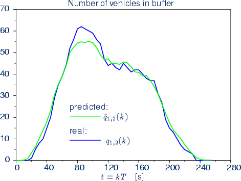
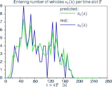
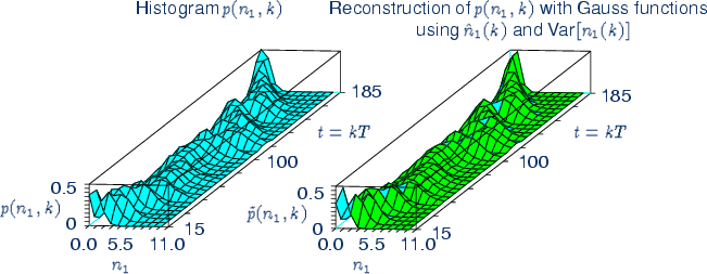
The critical probabilities are:
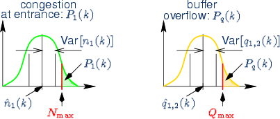
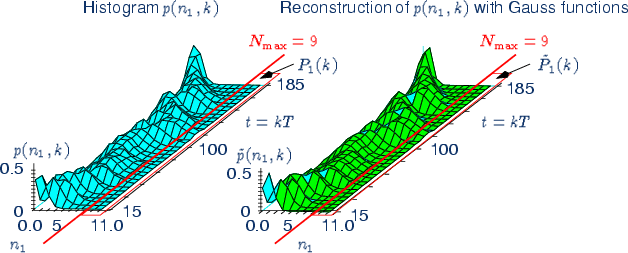
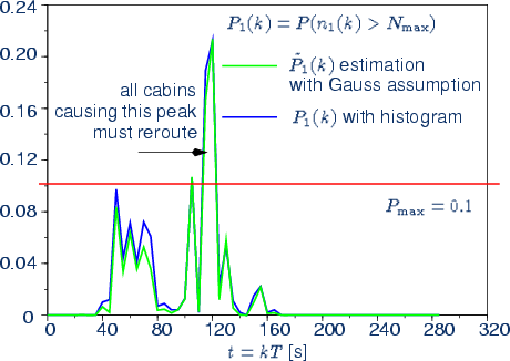
PSNC allocation criteria: if there exist a future
time-slot k for which
![]()
then any new allocation for this times-lot is refused or
rerouting/reallocation is requested.


Next: Bibliography

MAIT home
Last updated: 2001-05-30 by
webmaster@maitint.org