Subsections
3 Short Tutorials
Go through these tutorials if you are using the simulator for the
first time, they help you to quickly get a simulation designed and
running. For professional studies the advanced topics in
Sec. 4 are highly recommended.
Start up
iTS MAITin GUI mode (GUI= Graphical user interface) by typing
python its.py behind the terminal prompt or by double clicking
on the its-snake in your file browser. Then you should see the empty
main window as shown in Fig. 2. Now you can
continue with one of the short tutorials below.
Figure:
iTS MAITMain window
 |
3.1 Opening, starting and viewing simulation files
Choose from the main menu File / Open. You will always be asked
whether you want to save the present simulation. Press ``NO'' if
there is no simulation or if you have just saved it. Select the
simulation file fiera_users.its and press the ``OK'' button.
After the transportation network has appeared in the main window
(similar to Fig. 3), choose from the main menu
Simulation / Start. The vehicles and users should now start
moving. Stop the simulation with menu Simulation / Stop. You
can continue the simulation with
Simulation / Continue.
If you select again Simulation / Start the simulation will apparently
continue, but time and all statistical data will be set to zero.
There is also a step-by-step simulation option: click somewhere in the
canvas and press the return key. For each return-key
hit, the simulator will advance 500ms. Before continuing the
simulation in normal mode, you need to set the End of
simulation time to a desired value by selecting
Simulation / Parameters.
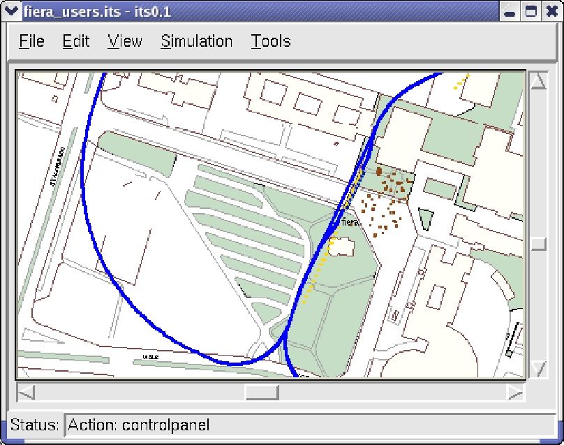
Figure 3:
The simulation fiera_users.its. The brown dots beside
the off-line stop are people (users) who will have a ride. The
vehicles are the yellow rectangles.
 |
Use the scroll-bars or cursor-keys to scroll the viewing area
of the canvas. Zoom in and out with the PgDown and PgUp
buttons.Attention: for large maps, enlargements are
computationally intensive and require a huge amount of memory!! More
zoom options are available on the View Menu. Choose View / indicate
ghosts to visualize how vehicles are merged and
de-merged. Attention, this option will slow down the display.
Network evaluation methods are explained in Sec. 3.2,
for Network creation and editing see Sec. 3.3.
3.2 Network evaluation
Open a complete simulation file (including vehicles and users as
demonstrated in Sec. 3.1) and simulate it for at least
10 minutes (see status bar below canvas). There are currently the
following methods available to evaluate the current state of the
simulation:
- The Control-panel
- is an interactive graphical user interface
which displays various information about a selected module (see
Fig. 4 with an example of a track element).
Figure 4:
The Performance page of the control-panel of a track element.
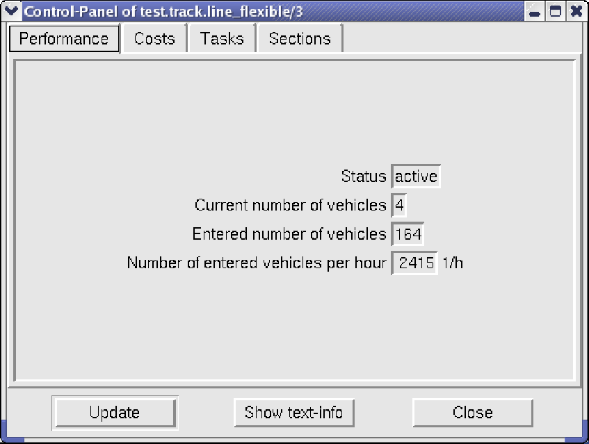 |
The information are ordered by subjects (for example performance,
costs, etc.) and presented on different pages which can be chosen on
the top border of the control-panel window. Many fields and buttons
are interactive, values can be changed by:
- clicking in the field,
- modifying value with keyboard and
- pressing the RETURN or ENTER button.
There are many possibilities to open control-panels:
- Select Edit/ Module/ Control-panel and click on a
module (user, track-element) within the canvas.
- Select Edit / Browse.... This will open a window with
a list of all simulation objects, also the ``hidden objects'' (for
example managements), which are not visible on the canvas. Select
an object and press the Control-panel button. Some objects contain
a number of individual modules of the same type (for example the
object base.user.test_driver contains all users of the type
``test-driver''). These modules are displayed on the right. In
this case, select one of the modules and press the Control-panel
button. A double click has the same effect as pressing the
Control-panel button.
- The control-panel can also be opened from within other
control-panels if there is a list-box with module names. For
example, there is a list of vehicles in the Section page
of each track element which are currently on the selected section
(select a section in the section list to show vehicles). Click
directly on the vehicle ID to open the control-panel of the
respective vehicle.
- Export results
- allows to write structured information about the
state of the simulation into a file. Currently the data is written
in table-form using a tab-separated text format. The resulting
file can be directly imported into text processing documents or
spread sheet applications.
Figure 5:
Example of file with exported results, when imported in a
spread sheet (here kspread from
KDE e.V).
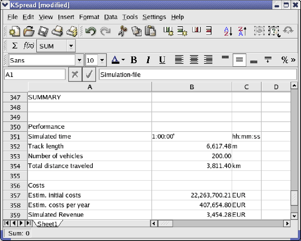 |
To export results, select Tools / Export results... from the
main menu, insert a file name with extension (for example .txt) in
the upcoming dialog-box and press OK. When imported with the
spread-sheet application kspread
(KDE e.V) the data looks as
shown in Fig. 5.
- Export canvas:
- see Sec. 3.4.
3.3 Designing an automated transport network
These are step-by-step instructions on how to design a network from
scratch. It is highly recommended to follow these
instructions at least for the first time you create a network. Keep
in mind that this is not a fully-developed commercial software with
all the conveniences like undo, group, mark, copy, paste, etc.
Furthermore, some parameters cannot be changed in later design steps
and need to be set at the beginning. However, following the
instructions below even larger networks can be rapidly and
conveniently designed, see also design sequence in
Fig. 6:
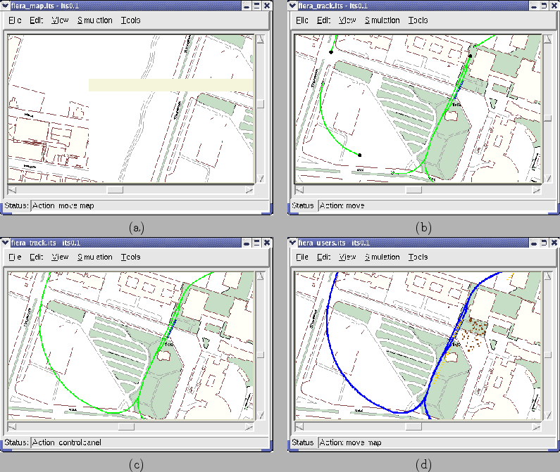
Figure:
Example of a step-by-step network design.(a) Moving and
placing background maps. (b) Placing stops and other track
element. (c) Closing the gaps with ``flexible'' track elements. This
design step is available in the its-0.51distribution, just open
simulation file fiera_track.its. (d) Track is ``activated''
and carriers as well as users have been added to the stops. The
simulation is now ready to run.
 |
- Create a new simulation with File / New from the main menu.
- Optionally, change currency in Simulation / Parameters (default
is EUR). Confusing results may occur when changing the currency
later.
- Optionally, put one or more scanned maps on the canvas: Select
Edit/ Map/ Add... from the main menu, select the graphic
file with the desired map in the browser-dialog window and press OK.
You should see the map on the canvas, attached to the pointer. Move
map to the correct position and place it with a click. The
add-and-place operation can be repeated for any number of maps.
Note that
iTS MAITis a micro-simulator, showing the movement of
individual people and vehicles. This means the map's resolution must
be high enough to show structures such as individual houses or cars,
which requires considerable memory and processing time for map
images. In order to obtain realistic results using maps, please read
carefully the following instructions:
- Scale the map to one pixel-per-meter (for example if
you want to include a 5km
 large map than it must have
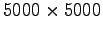 pixels
 pixels). This scaling is not
done by the simulator, it is required that you do this with a
graphics program before including it in the simulator. Note
that the width of vehicles, track and persons is slightly
over-sized (roughly factor 1.3) in order to improve visibility at
100% viewing scale.
pixels). This scaling is not
done by the simulator, it is required that you do this with a
graphics program before including it in the simulator. Note
that the width of vehicles, track and persons is slightly
over-sized (roughly factor 1.3) in order to improve visibility at
100% viewing scale.
- Save the map in GIF-format into the same directory as the
simulation file, default is
its-0.51/projects.
- Multiple background maps are recommended if the target area is
not rectangular. Try to avoid ``empty'' map space as maps
occupy a lot of memory, disk-space and slow down zoom
operations.
Hint:If you are designing a bigger network
it may be useful to delete all maps after designing the layout of
the network and before running the simulation. This will reduce
the memory occupation and increase simulation speed (in particular
zoom operations). However, keep a copy of the the simulation with
the maps in case you want to redesign/expand the network.
- The maps are not included into the simulation file (only their
names are). This saves you a lot of disk space but if you want to
copy the simulation for a friend, make sure to copy all map files
as well and do not change their names or location once they are
included.
- Best suited are aerial or satellite photographs of the target
area. Road maps have the disadvantage that the streets are drawn
wider than they are in reality. Aerial photographs give also a
more realistic impression when presenting a demo-simulation.
- For your convenience: Some menus have a dashed separator on the
top (for example Edit / Module). This means they can be torn-off and
placed permanently anywhere on the screen as permanent window. Just
select this separator to transform the menu into a window.
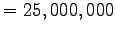
Figure 7:
The module browser. A selection panel for adding
track-elements, vehicles and users. To see this panel go
Edit/ Module/ Add...
 |
- Add, adjust and connect track elements: Open first the Module
browser with Edit/ Module/ Add.... The module browser, as
shown in Fig. 7, has a group-pull down menu and
module selection dialog box. Choose track-elements at the
group pull down menu. Select a particular track element
from the Modules selection box that you want to add to the
simulation. An example of a selected type is shown in the preview
window together with some additional text information. Note the
little circles on each extremity of track elements. An empty circle
indicates an input node (where vehicles enter), whereas a filled box
marks an output node (where vehicles leave).
Press the Select of the module-browser bottom and move
pointer over canvas (alternatively, double click on the module
type). The selected track element should now be attached to the pointer.
As long as the track element is attached to the pointer with one of
its nodes, the following operations can be used:
When creating the network, it is recommended to minimize the number
of track elements. This will considerably improve simulation speed.
This means: use few track elements and connect them by stretching
their extremities. This step requires a bit of experience. However,
with the following hints one can rapidly build up a network:
- Place first all stops. Maybe you have done some traffic demand
analysis of the target region and you know the rough position and
capacity of the stops. Make sure that the orientation (adjust with
``a'' and ``A'') is right and input nodes (open circles) and
output nodes (filled circles) are at the desired extremities of
the stop.
- Place diverge and merges elements with curves, circular
curves, and line elements wherever possible.
- Change radius and length of existing elements in order to
cover the maximum possible path:
- Go in move-mode by right-click when placing or by selecting
the Edit/ Module/ Move menu.
- Click on the node you want to move or stretch.
- Move the mouse to change shape of track element.
- Left-click to complete operation.
Stretching can also be used to make connections, when a filled and
empty node are close enough together.
- WARNING: there is currently no design rule checker!
You must make sure that the entry sections of all merges are
sufficiently long, this means length greater than
 , where
  is maximum comfort
deceleration,
is maximum comfort
deceleration,  is the brake actuation time and
  the
maximum line velocity.
the
maximum line velocity.
The nominal line velocity is a property of the section and can be
changed on the control-panel's Section-page. However,
nominal line velocity is not maximum line velocity. If the
previous section has a higher nominal line velocity then you must
leave the vehicles additional space to reduce their speed to adapt
to the nominal line velocity of the merge section. Do never
increase the line velocity of stops, otherwise they are no more
safe.
The accelerations are a property of carriers and can be changed on
their control-panel.
- Place diverges and merges with flexible extremities.
- Use again the move-mode to stretch the track elements and to
close as many gaps as possible by making connections. Pay again
attention to the length of the entry sections of merges.
- Close remaining gaps by placing and stretching flexible
lines.
- An alternative to adding track elements one can ``clone''
existing elements by selecting the
Edit/ Modules/ Clone tool and by clicking on the
track elements to be cloned. This is similar to the copy/paste
operation of text editing applications. The
Edit/ Modules/ Delete tool allows to delete
track-elements.
- Optionally, configure track-elements:
- Select Edit/ Modules/ Control-panel and click on
a track-element of the canvas.
- Click on the Sections page, and select an individual
sections of the track-element on the table of all sections. Change
nominal line velocity for the selected section. Do not forget to
hit the RETURN or ENTER key after editing a number in order to
make the changes valid for the simulator.
Attention, if you want to changes velocities then it is
absolutely required to read the warnings of the previous design
step, in particular concerning the merge elements. It may happen
that you must extend the entry section of a merge when increasing
the speed!!
Figure 8:
The costs page of the control-panel of a track element.
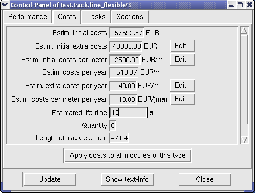 |
- Click on the Costs page of the control-panel, as
shown in Fig. 8. You see a list of
costs plus life-time and some other relevant quantities:
- Estim. initial extra costs
 All initial investment costs
which are not proportional to the track length (extra poles and
structures, elevators, etc.). This cost item can be edited in a
quantity/cost table by pressing the Edit... button, see
Fig. 9. The quantity is here the number of
this type of track element in the current network, which will be
automatically determined when calculating the costs.
All initial investment costs
which are not proportional to the track length (extra poles and
structures, elevators, etc.). This cost item can be edited in a
quantity/cost table by pressing the Edit... button, see
Fig. 9. The quantity is here the number of
this type of track element in the current network, which will be
automatically determined when calculating the costs.
- Estim. initial costs per meter
All initial investment
costs proportional to the track length (rails, beam-structure,
poles, etc.). This cost item can be edited in a quantity/cost
table by pressing the Edit... button. The quantity is here
the length in meter of the total network.
- Estim. extra costs per year
All annual operating
and maintenance costs which are not proportional to the track
length (control, cleaning, painting, repair). This cost item
can be edited in a quantity/cost table by pressing the
Edit... button. The quantity is here the number of this
type of track element in the network.
- Estim. costs per meter per year
All annual
operating and maintenance costs proportional to the track length
(cleaning, painting, repair). This cost item can be edited in
a quantity/cost table by pressing the Edit... button. The
quantity is here the length in meter of the total network.
- Estim. initial costs
Estim. initial extra costs
 Estim.
initial costs per meter
Estim.
initial costs per meter  length of track-element. This
cost item is a function of other costs and cannot be edited.
length of track-element. This
cost item is a function of other costs and cannot be edited.
- Estim. costs per year
Estim. extra costs per
year
Estim. costs per meter per year
length of
track-element. This cost item is a function of other costs and
cannot be edited.
- The life time can be changed directly in the text box, but
has currently no further use.
Figure 9:
Cost-table editor allows automatic economy of scale
calculations for network.
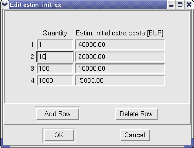 |
Press the Apply-button to apply costs to the present
track-element or the ``Apply costs to all modules of this
type''-button to copy the costs to all track-element of the
same type that exist in the entire network.
- In case of stops, you can click on the Parameters page of the
control-panel. The following parameters can be modified:
- Name of the stop. By default the simulator gives
unique numbers to the stops. If you want to give names to stop,
try to avoid whitespace! These names may be compared later with
the names in your origin-to-destination demand pattern table and
a stop-name with two space-characters is different from a name
with a single space-characters. You could use underscores
instead, use kings_road for example instead of kings
road
- Zone: You can also assign the stop to a so called
``zone''. The concept of zones is later used to add vehicles
and users. For example 50 users or vehicles can be distributed
over all stops which are in the same zone. The default zone of
all stops is maintenance.
- Berths to be kept clear: This is the desired number of
berth to be kept clear for newly arriving vehicles. This means
an empty vehicle will not be diverted into the stop if the
number of free berth is below the number specified in this
field. Default is that half of the berth must be kept clear.
The above parameters can be changed at any design step, but it is
recommended to do it before starting the simulation. Otherwise the
obtained simulation results are produced with a changing set of
system parameters.
- Save track layout! You will definitely want to change
your track later on. For this reason it is a good idea to save this
intermediate result now because after the next steps it becomes
increasingly difficult (and sometimes impossible) to remove vehicles
and users from the simulation in order to get back to the plain
track. Therefore, Select File / Save as... on the main
menu and insert the name of the simulation. The suggested name is
mycity_track.its, to indicate that this simulation file
contains track information only.
- Activation of track elements: The activation of track elements
is somehow similar to switching on the real track after
installation. To activate the track go to menu item
Edit/ Module/ Activate. Then click on the track element
that you want to switch on. Alternatively you can activate
the entire network at once with Edit/ Module/ Activate all.
Note: Only track elements that are connected on all nodes can
be activated. However, single section of a track element can be
activated if both ends are connected. Furthermore, only inactive
track elements can be moved, stretched or deleted. For inactivation
go Edit/ Module/ Inactivate and click on the track
elements to inactivate.
- Add vehicles: click on module-browser and select Carriers
(carrier is MAIT terminology). You could double-click on a carrier
type (currently only experim is available), drag it over a
stop on the canvas and click to place it into a berth. However, a
more effective method is to select a carrier and press the Add
multiple bottom. A dialog box will appear with the following
options:
- Number of vehicles to be added
- The zone to where the vehicles are distributed. The default is
everywhere.
- Maximum absolute comfort, emergency and failure acceleration
rates.
The emergency and failure deceleration define the minimum
achievable headway dependent on velocity.
The headway in turn will ultimately limit line capacity, see
discussion in Sec. 5.3.
You can repeat this operation to place any amount of vehicles to
stops in different zones.
- Optionally, edit costs of carriers: Select
Edit / Browse..., and test.car.experim in the
simulation objects list. Click on any particular carrier in the
Modules list and press the Show control-panel-button. Click
on the Costs page of the control-panel. You will see a
lists of costs plus life-time and some other relevant quantities:
- Estim. initial costs
All initial investment costs This
cost item can be edited in a quantity/cost table by pressing the
Edit... button. The quantity is here the number of this
carrier type in the current network.
- Estim. costs per year
All annual operating and maintenance
costs (control, cleaning, painting, repair).This cost item can
be edited in a quantity/cost table by pressing the Edit...
button. The quantity is here the number of this carrier type in
the current network.
Press the Apply-button to apply costs to the present
carrier or the ``Apply costs to all modules of this
type''-button to copy the costs to all carriers of the same type
that exist in the entire network.
- It is recommended to save the state of the simulation file after
adding vehicles with the name mycity_cars.its
- Add users: click on module-browser window and select Users. For this exercise we will select the user `` test_driver''. Double-click on test_driver, drag him/her
close to a stop on the canvas and click to place. However, a more
effective method is to select the test_driver in the browser
window with a single click and press the Add
multiple bottom. A dialog box will appear with the following
options:
- Number of users to be added
- The zone to where the users are distributed. The default is
everywhere.
- The boarding time, including door opening entering the
vehicle and door closing.
- The exit time. Same as boarding time, but passenger leaves the
vehicle.
You can repeat this operation to place any amount of test drivers to
stops in different zones.
- Optionally, change End of simulation time in
Simulation / Parameters (default is
 ).
).
- It is recommended to save the state of the
simulation file after adding users with the name
mycity_users.its
- Run simulation with Simulation / Start.
3.4 Graphics export and printing of canvas
Unfortunately there is currently no platform-independent printing
scheme for graphics implemented. However, there are two methods to
export the transport-network in a printable graphics format:
Postscript snapshot and screen-shots.
Postscript(R), is the Adobe(R) file-format for printers. You may be
able to drag and drop a postscript file directly into a postscript
compatible printer symbol, on almost all Unix systems you simply type
at the prompt: lp postscriptfile.ps and the file will be printed
directly to the postscript line printer or automatically converted to
a proprietary format and then printed.
Postscript files can also be viewed and edited. There is commercial
software, such as Adobe Acrobat Distiller/Reader and Photoshop. The
most widespread free software is Ghostview and the Gimp. Windows users can
download the free software at

To make postscript snapshots, simple select Tools / Make PS
snapshots. If you now run the simulation, a snapshot will be made
every  by default. The files will be saved in the current
directory under the name(s): mysimfile_shot001.ps, mysimfile_shot002.ps, mysimfile_shot003.ps,
by default. The files will be saved in the current
directory under the name(s): mysimfile_shot001.ps, mysimfile_shot002.ps, mysimfile_shot003.ps, 
Note: the PS snapshots cover only the area of the canvas that you
actually see in the window on the screen (but without window
borders). If you want the whole network, you may want to zoom out
first.
Screen-shots are probably the quickest and simples way to export graphics:
- MS windows:
- Maximize window with canvas.
- Press the ``Print Screen''-key
- Open MS Paint or other MS text/graphics applications
- Select Edit / Paste, or in MS word
Edit / Paste Special....
- Optionally, edit graphics (cut off windows frame and menu,
resize, compress, etc.)
- Linux:
- Maximize window with canvas.
- Take a snapshot using your favorite snap-shooter (for example
ksnapshot that comes with the KDE desktop) and save window as
graphics file.
- Optionally, edit graphics with gimp (cut off windows frame and
menu, resize, compress, etc.)
Joerg Schweizer
2007-07-17