Next: 6 Bugs Up: The Innovative Transportation Simulator Previous: 4 Advanced topics
The simulator as a whole is a complicated piece of software with many interacting objects. Even though details of the internal functions are hidden away behind a graphical user interface, it may be required to have a minimum understanding of the simulator's operating principles.
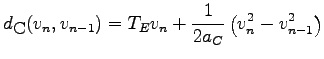
The basic principle of the simulator is quite simple: a simulation consists of a set of simulation objects. Each object contains:
The methods to change the internal state of objects or modules are event-driven. There are principally two types of events:
 |
All (relevant) simulation objects and modules can be listed and inspected with the object browser: Select Edit / Browse.... As it can be seen in the lists, simulation objects as well as modules have unique identifications (IDs). The naming scheme for simulation objects is:
The naming scheme for modules is composed of the parent simulation object ID plus a serial number:
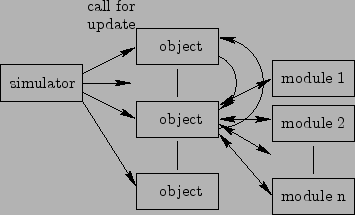
This section gives an overview of the functions of simulation objects and modules and their relation to other objects, see Figure 11.
 |
The vehicle-follower control algorithm is currently more optimized for simulation speed rather than for precise/optimized motion control. This means the following differences compared with a realistic control system: (i) there are no jerk-limits (in neither direction); (ii) speed changes of the first vehicle in a vehicle chain is almost instantly and fully propagated through the chain, which results in a reduced ride comfort; Differences (i) and (ii) result in a slightly higher line capacity of the simulated system compared with a real system.However additional time headway, necessary for jerk adaptation and be simulated by increasing the brake actuation time, which is one parameter of carriers.
Speed-limits, maximum comfort/emergency/safet acceleration are respected. All parameters can be modified via Add multiple bottom or control-panels.
All managements together (see Fig. 11) perform the logistics of the network by exchanging information among each other, but also with the physical world (track-elements, carriers, users).
Apart from standard administrative operations, the managements currently optimize only the trip-time: They route the vehicle to its destinations on a path that has the shortest expected trip-time. If a branch is blocked, the vehicle is deviated, which will trigger a rerouting. Empty vehicles will be ``intelligently'' routes to the nearest stop with a higher user-demand.
If there is are no passengers at a stop, empty vehicles are send into the network. An empty vehicle is branched into a stop if there are waiting passengers at this moment. There is currently no predictive resource allocation--not for vehicles and neither for the network. This means traffic congestion can occur if the network has a bottleneck.
The organization of the entire logistic is based on the creation, exchange,and execution of tasks: If a management wants to get a service performed by a target (another or the same management or physical module), it must send an order. When the target receives the order, it will create a task for this order. The task inside the target will create one or several actions (or create orders for other managements and/or modules) which are necessary to fulfill the task. The task persist in the target until it is terminated, failed or explicitly killed. In either way the task will report the results to the entity which created the order.
Tasks are the instrument to control the network globally on large time scales. They are the bases for doing distributed, parallel computing in the system's heterogeneous computer network. Note that tasks are a inherent feature of most operating systems. The concept of tasks used in the simulator has been designed to fulfill the special requirements of the transportation network, including physical objects and a multi-level management. In later versions the simulation objects (in particular the management objects) could run on different processors, using the task mechanism of the respective operating system.
The task page of each control-panel shows task ID, status, the order ID and the object/module which created. Modules have usually only one task at a time, management units must handle many tasks simultaneously.
Before explaining the simulated system, a few words to the general PRT control-problem. A controller for short time head-ways needs to meet simultaneously criteria for safety, string stability, comfort and speed transitions.
The safety criteria can be expressed by means of the
minimum safety distance
![]() between vehicles that is
required to avoid a collision between two consecutive vehicles.
In general,
between vehicles that is
required to avoid a collision between two consecutive vehicles.
In general,
![]() is proportional to the difference between the
squared velocities of follower and lead-vehicle. In many control
schemes, the level of safety is given by the safety factor
is proportional to the difference between the
squared velocities of follower and lead-vehicle. In many control
schemes, the level of safety is given by the safety factor
![]() when the actually achievable distance is
when the actually achievable distance is
![]() .
.
String stability means that a speed change of a vehicle in the string decreases in magnitude when propagating through the following vehicles.
The comfort criteria sets usually limits to the maximum allowed
man![]() ver accelerations and jerks.
ver accelerations and jerks.
Speed transitions do occur during various vehicle man![]() vers,
such as approaching, following, merging, diverging, stopping or
velocity changes. It is obviously required to guarantee all
the above criteria during all possible speed transitions. One specific
transition criteria is the ``fixed end-point speed transition''(FEPST)
criterion:all vehicles in the string must be at the lower safe speed at a
fixed point of the track, not just the first vehicle.
vers,
such as approaching, following, merging, diverging, stopping or
velocity changes. It is obviously required to guarantee all
the above criteria during all possible speed transitions. One specific
transition criteria is the ``fixed end-point speed transition''(FEPST)
criterion:all vehicles in the string must be at the lower safe speed at a
fixed point of the track, not just the first vehicle.
The optimization criteria for lateral-controller is usually to
maximize the line capacity or to minimize head-ways. The theoretical
limits of carrying capacity and safety-level are generally set by the
adopted vehicle spacing policy. The relevant policies are
the constant time headway policy and constant safety policy.
Constant time headway offers a constant, speed independent carrying
capacity, while the safety factor drops below unity as velocity
increases. Constant safety spacing guarantees a
![]() . But for
higher velocities, the carrying capacity drops below the one of the
constant time headway spacing.
. But for
higher velocities, the carrying capacity drops below the one of the
constant time headway spacing.
Now we introduce the necessary parameters and math: If vehicle ![]() has a maximum failure deceleration of
has a maximum failure deceleration of ![]() and the following vehicle
and the following vehicle
![]() can guarantee an emergency deceleration of
can guarantee an emergency deceleration of ![]() by applying the
emergency brake after time
by applying the
emergency brake after time ![]() then vehicle
then vehicle ![]() is in a safe state
if
is in a safe state
if
![]() with
with
Parameters ![]() ,
, ![]() ,
, ![]() , vehicle length
, vehicle length ![]() and the nominal line velocity
and the nominal line velocity
![]() do ultimately determine the line capacity
do ultimately determine the line capacity ![]() in vehicles per hour, with
in vehicles per hour, with
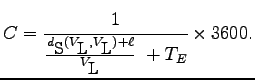
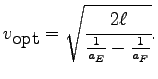
The nominal line velocity
The comfort criteria is introduced by limiting the acceleration
![]() of each vehicle
of each vehicle ![]() at the comfort acceleration
at the comfort acceleration ![]() . If we
want to avoid collisions by braking only at at the comfort rate we
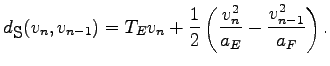
must respect the minimum comfort distance
. If we
want to avoid collisions by braking only at at the comfort rate we
must respect the minimum comfort distance
![]() with
with
The simulator can do both, constant safety and constant
time headway. In fact, constant time headway is a special case of a
constant safety, when
![]() . The controller of the simulator does
simply guarantee that the distance is at all times and for all
vehicles grater than both,
. The controller of the simulator does
simply guarantee that the distance is at all times and for all
vehicles grater than both,
![]() and
and
![]() . If there is no vehicle in front, the vehicle
will accelerate to the given nominal line velocity, which is a
property of the section of the current track element.
. If there is no vehicle in front, the vehicle
will accelerate to the given nominal line velocity, which is a
property of the section of the current track element.
Attention: at merge points you have to make sure that the legs of the merge element
are at least as long as
![]() , otherwise vehicle won't have the chance to
line up properly and crashes may occur.
, otherwise vehicle won't have the chance to
line up properly and crashes may occur.
All accelerations and the brake actuation time should be modified during the ``add multiple'' operation, when adding the carriers to the network. The parameters of individual vehicles can be modified through their control-panel.
The nominal line velocity can be modified for each section at the Sections-tab of the control-panel of each track-element. Section 4.4 explains how to do this.
There is also the possibility to introduce a comfort jerk ![]() :
simply add to the brake actuation time the term
:
simply add to the brake actuation time the term
![]() . This will add enough time-headway so that the
acceleration can adapt at comfort jerk rate in the worst case
scenario.
. This will add enough time-headway so that the
acceleration can adapt at comfort jerk rate in the worst case
scenario.
Joerg Schweizer 2007-07-17